I’ve got to admit that my relationship with Excel 2 years ago went as deep as SUMIF, AVERAGE and COUNT.
Therefore, I was an Excel noob.
Only in the past year, I started working with larger data sets on Excel. Therefore, I decided to level up my Excel skills.
Here are 6 Excel functions that I find most useful at work. Some are covered extensively online (I’ll not go through them). Some were difficult to find — I’ll explain these.
1. VLOOKUP (Vertical LOOKUP)
This is used to search a column for a value, and then return a value from another column in the same row.
This is the gist of it.
The VLOOKUP formula for the scenario below would be: =VLOOKUP(“Apple”, A:G, 7, FALSE).
“Apple” is the word you’re looking for, A:G is the range you’re looking at, 7 is the row number you want to retrieve your answer from, and FALSE means exact match.
Most of the time, we use FALSE.

Microsoft shows us how to use it here.
2. Turn non-dates into dates
Sometimes, Excel may not recognise your dates as dates. Especially when it comes with the time. You’ll know if you tried changing the format to “Short date” and nothing happens. Or if you performed a formula involving dates but you get 0.
When that happens, try this. First, remove the time by using this formula.

MID (A1, 7, 4) means from cell A1, take 4 characters starting from the 7th character.
This is to brute force your numbers to position themselves correctly.
At this point, it’s still not a date. We have to turn it into a date with another formula.
Here, we’re telling Excel that in cell B1, the second section is the month, and the third is the day.

Bonus: You can also use this formula when Excel gets the month and day wrong.
3. Set up a Forex sheet
In Google Sheets, you can use the formula =GOOGLEFINANCE(“CURRENCY:EURUSD”)*1000 to convert 1000 EUR to USD.
But in Excel, there’s no formula to convert currency. You’ll have to first set up a forex sheet to get the conversion rates. Then use these rates to convert your currencies.
4. Analyse data with Pivot Table
Pivot Tables are useful to get a quick summary of a large set of data. For example, I have a customer list with 4 columns:
- Customer_id
- Birthday
- Package or subscription
- Date of purchase
I can insert a Pivot Table to tell me things like:
- How many packages and subscriptions did we get in January?
- How many users were born in the first half of the year?
In real life, you probably won’t only have 4 columns. So there’re more complex analyses you can do with Pivot Tables.
5. Add UTMs to your URLs with CONCATENATE
CONCAT combines text from multiple cells into one cell. I use this to add UTMs or extra parameters to my URLs.
There are many URL builders online, but to store all your URLs in one sheet, this would be the best option.

6. Neaten up your sheet with IFERROR
If you take a value divided by nothing multiple times, you get a confused-looking sheet and a risk of getting fired for acquiring zero leads in 5 months.
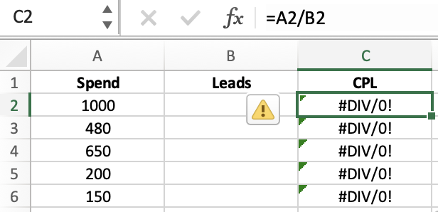
To clear up the confusion, use =IFERROR(your division, “”). This will return a blank cell.
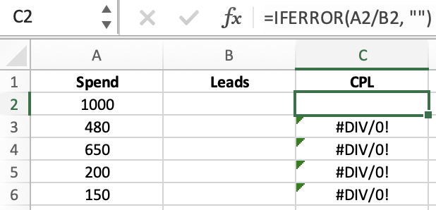
Or you can also use a hyphen instead =IFERROR(your division, “-”). This will return a cell with a dash.
That’s it. I’ll add more to this list if I come across any other formulas that saved my life. Hope it helps!